Build an End-to-End Lakehouse in Microsoft Fabric with Azure for Students

If you have a student email address, this guide is for you — especially if you want hands-on experience building an end-to-end data pipeline in Microsoft Fabric.

With an Azure for Students subscription, you receive ~$100 USD in free credits to spin up resources. In this tutorial, you will build a complete Medallion Lakehouse Architecture (Bronze → Silver → Gold) using Delta Lake and orchestrate the workflow using Fabric Data Factory Pipelines.

Note on Student Accounts: Azure F-SKU capacities below F64 require a Power BI Pro license to publish and view Power BI reports. Therefore, this project focuses strictly on the core Data Engineering pipeline: raw ingestion, PySpark cleaning, Delta Time Travel recovery, V-Order optimization, and pipeline orchestration.

Project Architecture

[ Built-in Sample Dataset ]
        │
        ▼  (Dataflows Gen2: Low-Code Ingestion)
[ Bronze Layer: bronze_orders ]
        │
        ▼  (PySpark Notebook: Cleaning & Normalization)
[ Silver Layer: silver_order ]
        │   └─► [ Delta History, Time Travel & RESTORE ]
        ▼  (PySpark Notebook: Aggregations & Performance Tuning)
[ Gold Layer: gold_fact_sales ]
        │   └─► [ OPTIMIZE with V-Order ]
        ▼
[ Data Factory Pipeline Orchestration ]

Part 1: Provisioning Fabric Capacity in Azure

1. Log in to the Azure Portal using your student email account.

2. In the top search bar, search for Microsoft Fabric and click Create.

   

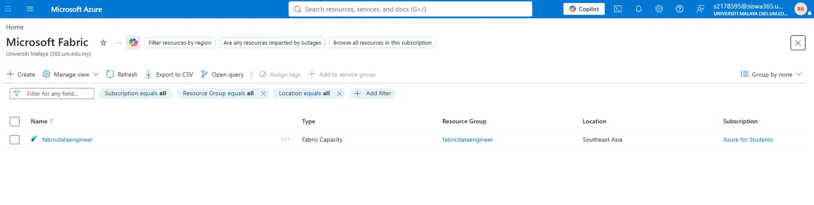
3. Fill in the required details:

   • Subscription: Azure for Students
   • Resource Group: Select or create a new resource group (e.g. rg-fabric-student).
   • Capacity Name: Enter a unique name (e.g. fabcapacitystudent).
   • Size: Select F2 (the smallest capacity unit available).
   • Tags (Optional): Add tags like Environment: Dev or Project: Fabric to track spending in Azure Cost Management.

   

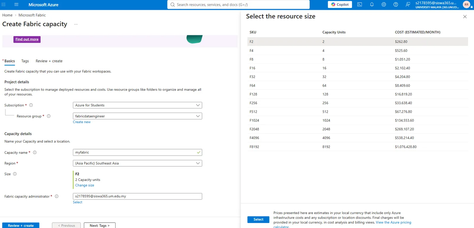
4. Click Review + create, then click Create.

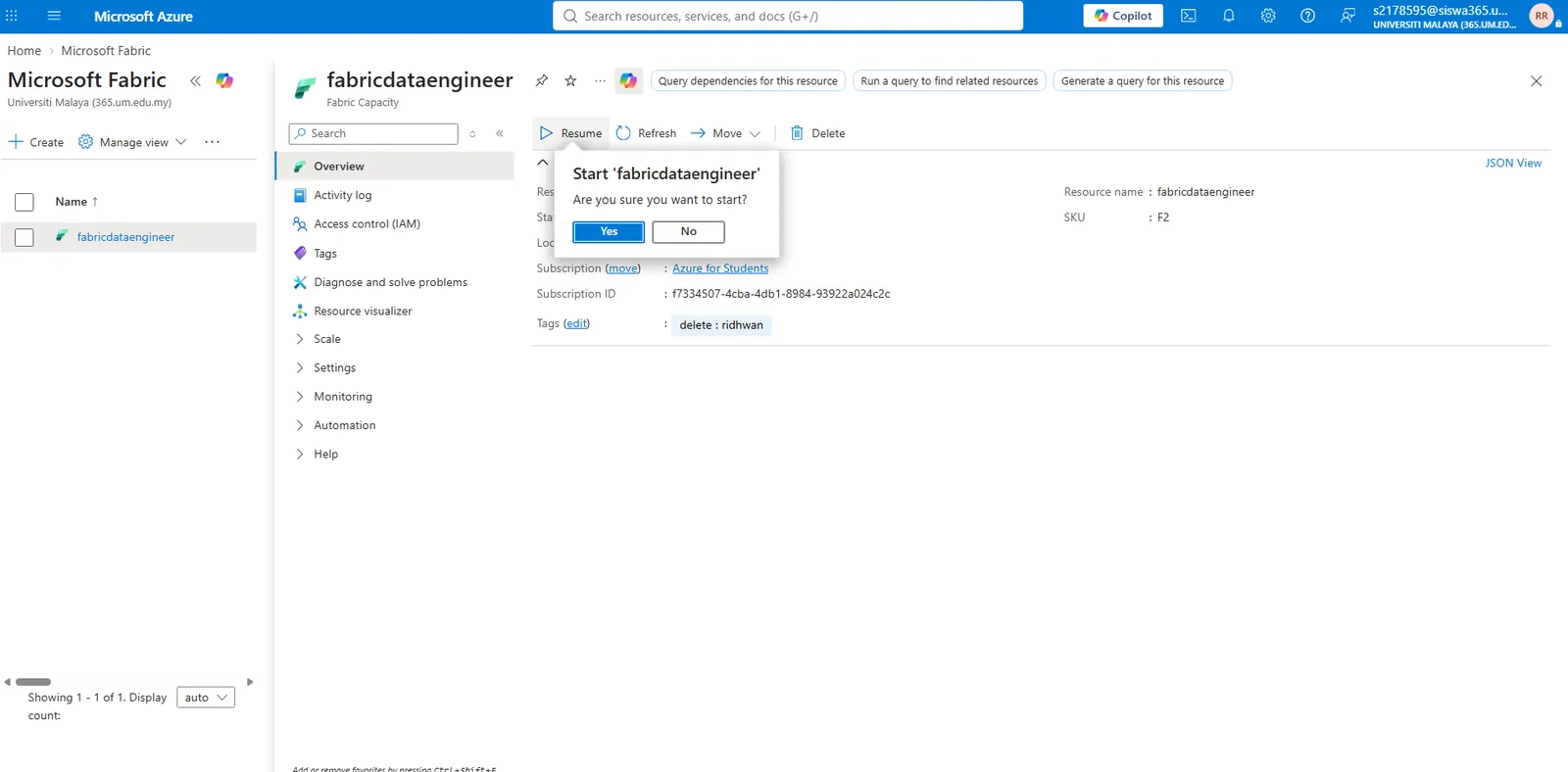
5. Once deployment completes, navigate to your new Fabric capacity resource. Notice that the capacity defaults to Paused to save your credits.

   

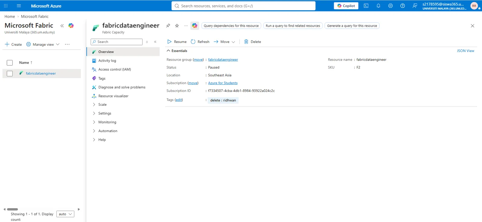
Part 2: Fabric Workspace Setup

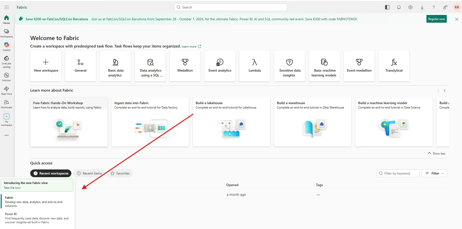
1. Open the Microsoft Fabric Portal in your browser using the same student email.

   

2. Click Resume on your Fabric capacity in Azure when you are ready to work. (Remember to pause it when you finish to avoid consuming your hourly credits!)

   

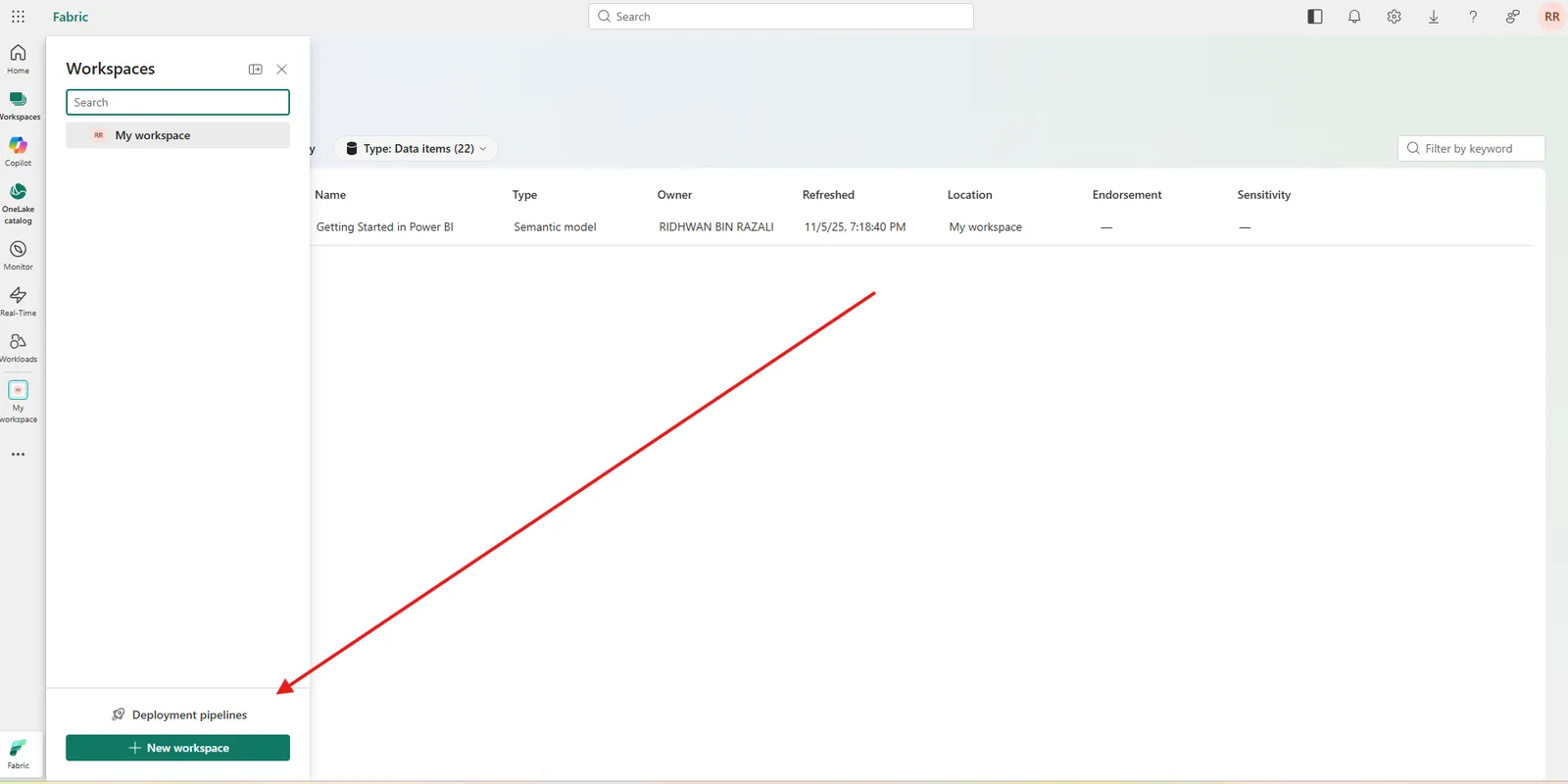
3. In the Fabric portal, click Workspaces on the left navigation bar, then select + New workspace.

   

4. Enter a name (e.g. ws_sales_analytics).

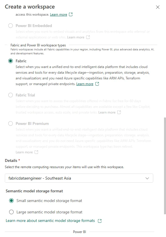
5. Expand Advanced, set the License mode to Fabric capacity, and select the F2 capacity you created in Azure.

   

6. Click Apply.

Step 1: Ingestion via Dataflows Gen2 (Bronze Layer)

In this step, you will use Dataflows Gen2 to ingest raw data from a public CSV file directly into your Lakehouse as a Bronze table.

1. In your workspace, click + New item → Dataflow Gen2.

2. Name the Dataflow df_ingest_sample_data.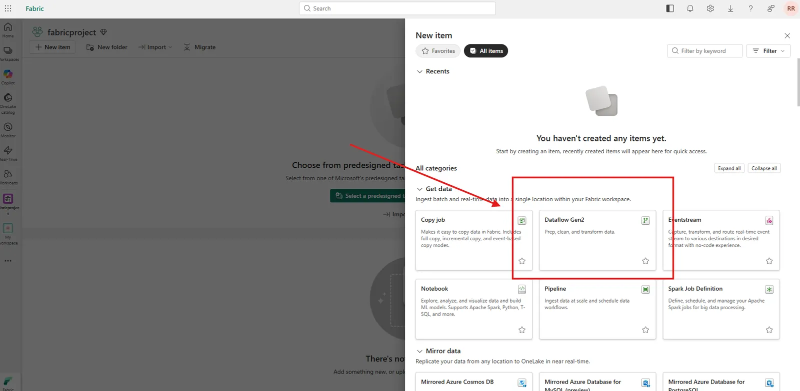

   

3. Select Import from a Text/CSV file and configure the connection:

   • File path or URL: https://raw.githubusercontent.com/MicrosoftLearning/dp-data/main/orders.csv
   • Authentication kind: Anonymous

4. Click Next to preview the file, then click Create.

   

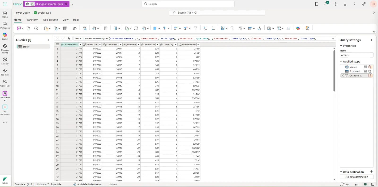
5. Add a Custom Transformation:

   • Select the Add column tab on the top ribbon.
   • Click Custom column.
   • Set New column name to MonthNo.
   • Set Data type to Whole Number.
   • Enter the formula: Date.Month([OrderDate])

   

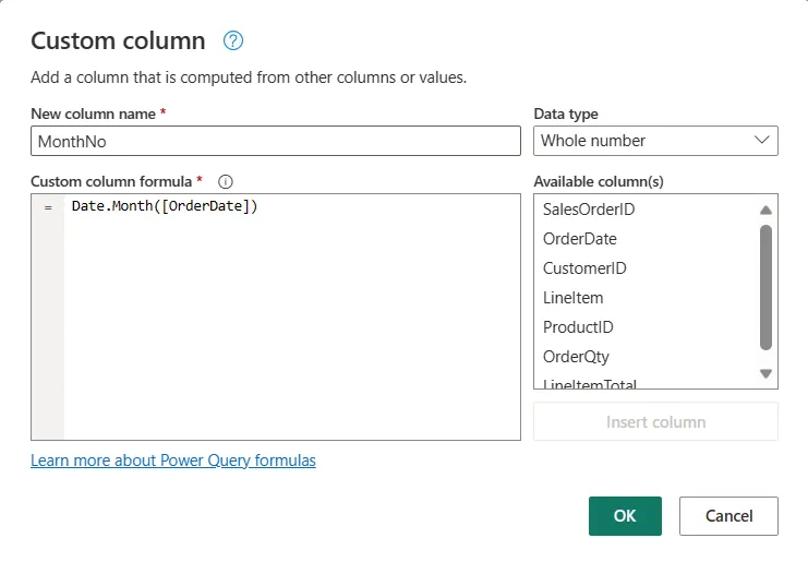
   • Click OK.

   

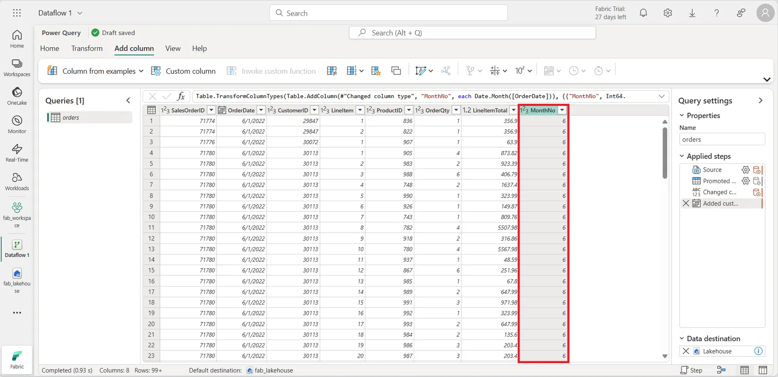
6. Set the Data Destination:

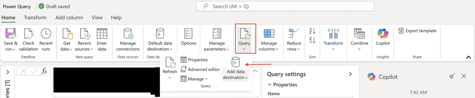
   • Select the Home tab, then click Add data destination → Lakehouse.

   

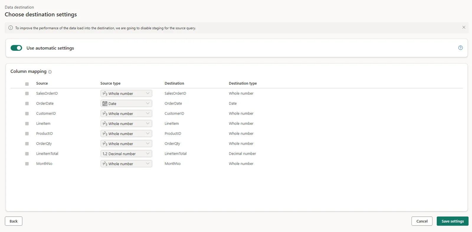
   • Connect to your workspace Lakehouse (create a new Lakehouse named sales_lakehouse if prompted).
   • Set the target table name to bronze_orders.
   • Ensure the update method is set to Replace.

   

7. Click Save & run at the bottom right corner and wait for the execution to complete.

Step 2: Silver Layer & Delta Time Travel Demo (PySpark)

Now, create a PySpark notebook to clean the raw Bronze data, enforce types, and write it out to the Silver layer. You will also demonstrate Delta Time Travel disaster recovery.

1. In your workspace, click + New item → Notebook.

2. Name it nb_01_silver_transform.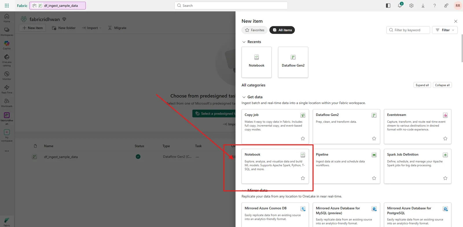

   

3. In the left Explorer panel, click + Add and attach sales_lakehouse.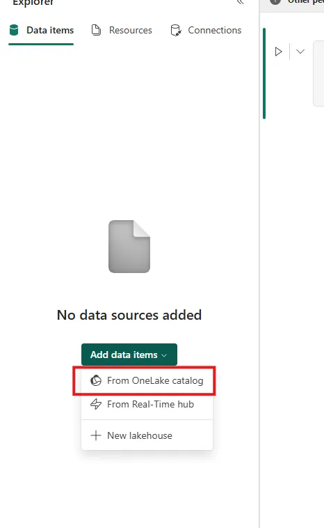

   

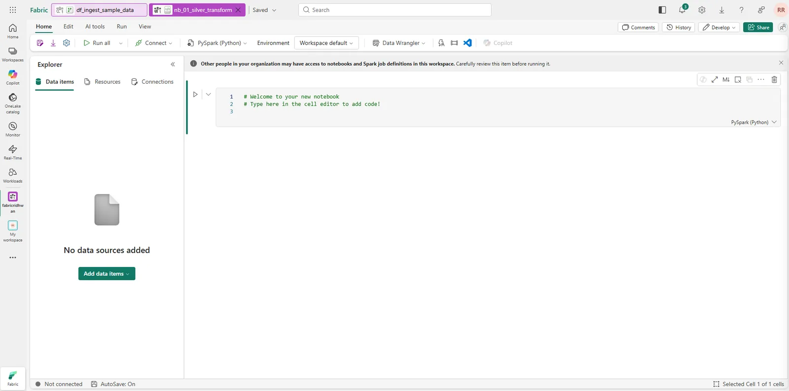
You will see your notebook after it is created.

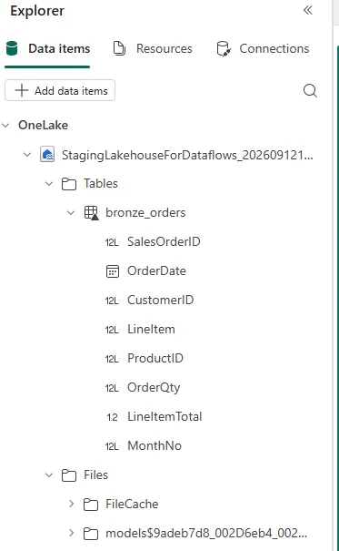
Now you can see the table on the left side.

1. Data Cleaning & Normalization

Add the following PySpark code block and run the cell:

from pyspark.sql.functions import col, trim, upper, current_timestamp, coalesce, lit, to_date
 
# 1. Read Raw Bronze Delta Table
df_bronze = spark.read.table("bronze_orders")
 
# 2. Clean, standardize data types, and add metadata columns
df_silver = df_bronze \
    .withColumn("SalesOrderID", col("SalesOrderID").cast("integer")) \
    .withColumn("OrderDate", to_date(col("OrderDate"))) \
    .withColumn("CustomerID", col("CustomerID").cast("integer")) \
    .withColumn("LineItem", col("LineItem").cast("integer")) \
    .withColumn("ProductID", col("ProductID").cast("integer")) \
    .withColumn("OrderQty", col("OrderQty").cast("integer")) \
    .withColumn("LineItemTotal", col("LineItemTotal").cast("double")) \
    .withColumn("MonthNo", col("MonthNo").cast("integer")) \
    .withColumn("IngestedAt", current_timestamp()) \
    .dropDuplicates()
 
# 3. Write Cleaned Data to Silver Layer
df_silver.write \
    .format("delta") \
    .mode("overwrite") \
    .saveAsTable("silver_order")
 
print("Silver layer successfully populated.")

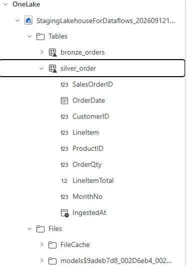
You will see the Silver layer table written on the left side.

2. Delta Time Travel & Recovery Demo

Delta Lake maintains an immutable transaction log (_delta_log) that tracks all table changes. Run this code block to simulate data corruption and recover the table using RESTORE:

# --- DEMO: Accidental Corruption ---
# Simulate a bug where LineItemTotal is mistakenly zeroed out
df_corrupted = spark.read.table("silver_order").withColumn("LineItemTotal", lit(0.0))
df_corrupted.write.format("delta").mode("overwrite").saveAsTable("silver_order")
 
# --- STEP A: Inspect Delta Commit History ---
display(spark.sql("DESCRIBE HISTORY silver_order"))
 
# --- STEP B: Query Historical Snapshot (Time Travel) ---
# Inspect data prior to corruption (Version 1)
df_version_1 = spark.read.option("versionAsOf", 1).table("silver_order")
print("Row count from valid Version 1:", df_version_1.count())
 
# --- STEP C: Restore Table to Valid Snapshot ---
spark.sql("RESTORE TABLE silver_order TO VERSION AS OF 1")
 
print("Table restored successfully to Version 1!")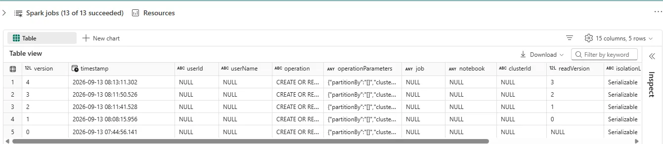

Note on Delta Retention: By default, Fabric retains Delta table commit history for 7 days. Background maintenance jobs (VACUUM) clean up older unreferenced Parquet files after this threshold.

Step 3: Gold Layer & Performance Optimization (PySpark)

In this step, aggregate the Silver data into a Star Schema (Dimensions & Fact tables) and apply Microsoft Fabric's proprietary V-Order write optimization.

1. Create a new Notebook named nb_02_gold_star_schema.

2. Attach sales_lakehouse on the left panel.

3. Paste and run the following code block:

from pyspark.sql.functions import col, year, month, quarter, date_format, current_timestamp
 
# -------------------------------------------------------------------------
# STEP 1: Enable V-Order globally for all writes in this Spark Session
# -------------------------------------------------------------------------
spark.conf.set("spark.sql.parquet.vorder.enabled", "true")
 
df_silver = spark.read.table("silver_order")
 
# -------------------------------------------------------------------------
# STEP 2: Write Dimension Tables with V-Order
# -------------------------------------------------------------------------
# Customer Dimension
df_silver.select("CustomerID").distinct() \
    .write.format("delta").mode("overwrite").saveAsTable("gold_dim_customer")
 
# Product Dimension
df_silver.select("ProductID").distinct() \
    .write.format("delta").mode("overwrite").saveAsTable("gold_dim_product")
 
# Date Dimension
df_silver.select("OrderDate").distinct() \
    .withColumn("DateKey", date_format(col("OrderDate"), "yyyyMMdd").cast("integer")) \
    .withColumn("Year", year(col("OrderDate"))) \
    .withColumn("MonthNo", month(col("OrderDate"))) \
    .withColumn("Quarter", quarter(col("OrderDate"))) \
    .write.format("delta").mode("overwrite").saveAsTable("gold_dim_date")
 
# -------------------------------------------------------------------------
# STEP 3: Write Fact Table with V-Order
# -------------------------------------------------------------------------
fact_sales = df_silver.select(
    col("SalesOrderID"),
    col("LineItem"),
    col("CustomerID"),
    col("ProductID"),
    date_format(col("OrderDate"), "yyyyMMdd").cast("integer").alias("DateKey"),
    col("OrderQty"),
    col("LineItemTotal"),
    current_timestamp().alias("IngestedAt")
)
 
fact_sales.write.format("delta").mode("overwrite").saveAsTable("gold_fact_sales")
 
# -------------------------------------------------------------------------
# STEP 4: Run Table Maintenance & Compaction
# -------------------------------------------------------------------------
spark.sql("OPTIMIZE gold_fact_sales")
 
print("Gold Star Schema created and optimized with V-Order.")

Understanding V-Order & OPTIMIZE

• V-Order: A proprietary write-time sorting algorithm in Microsoft Fabric. It restructures Parquet memory layouts so that reporting engines can read data directly into memory without overhead.
• OPTIMIZE Command: Consolidates small, fragmented Parquet files into larger files to prevent the "small file problem" common in distributed data processing.

Step 4: Pipeline Orchestration with Data Factory

Now chain all three components into an automated execution sequence using a Fabric Data Pipeline.

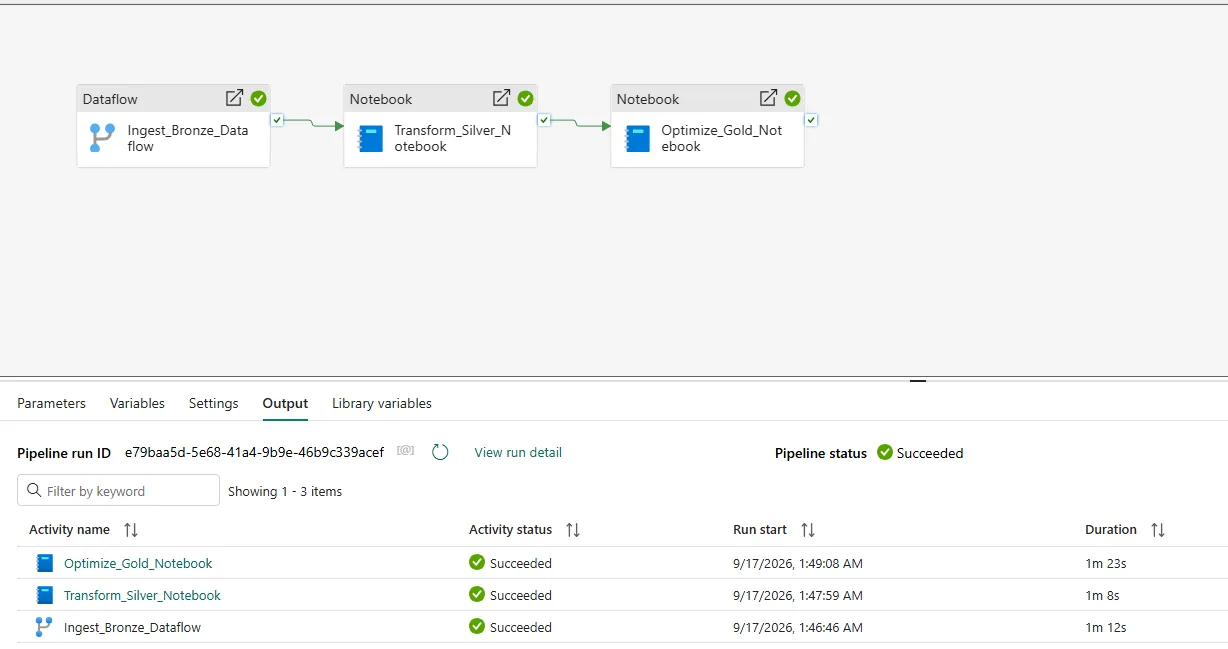
1. In your workspace, click + New item → Data pipeline.

2. Name it pl_master_sales_etl.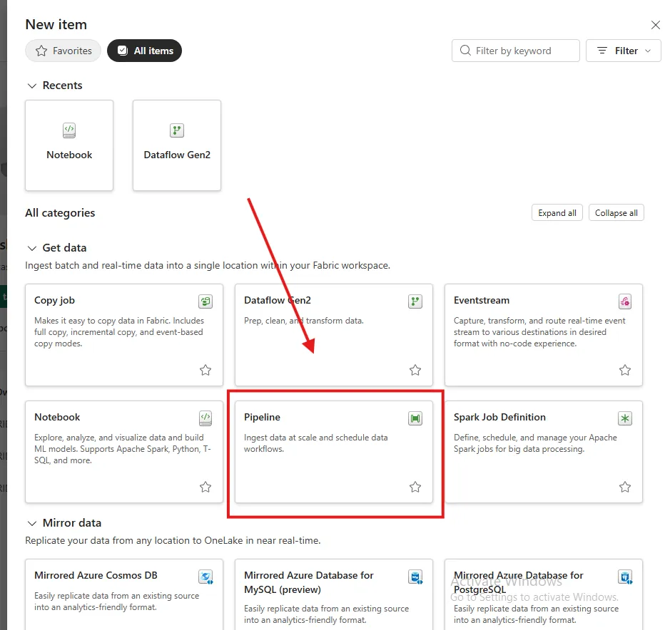

   

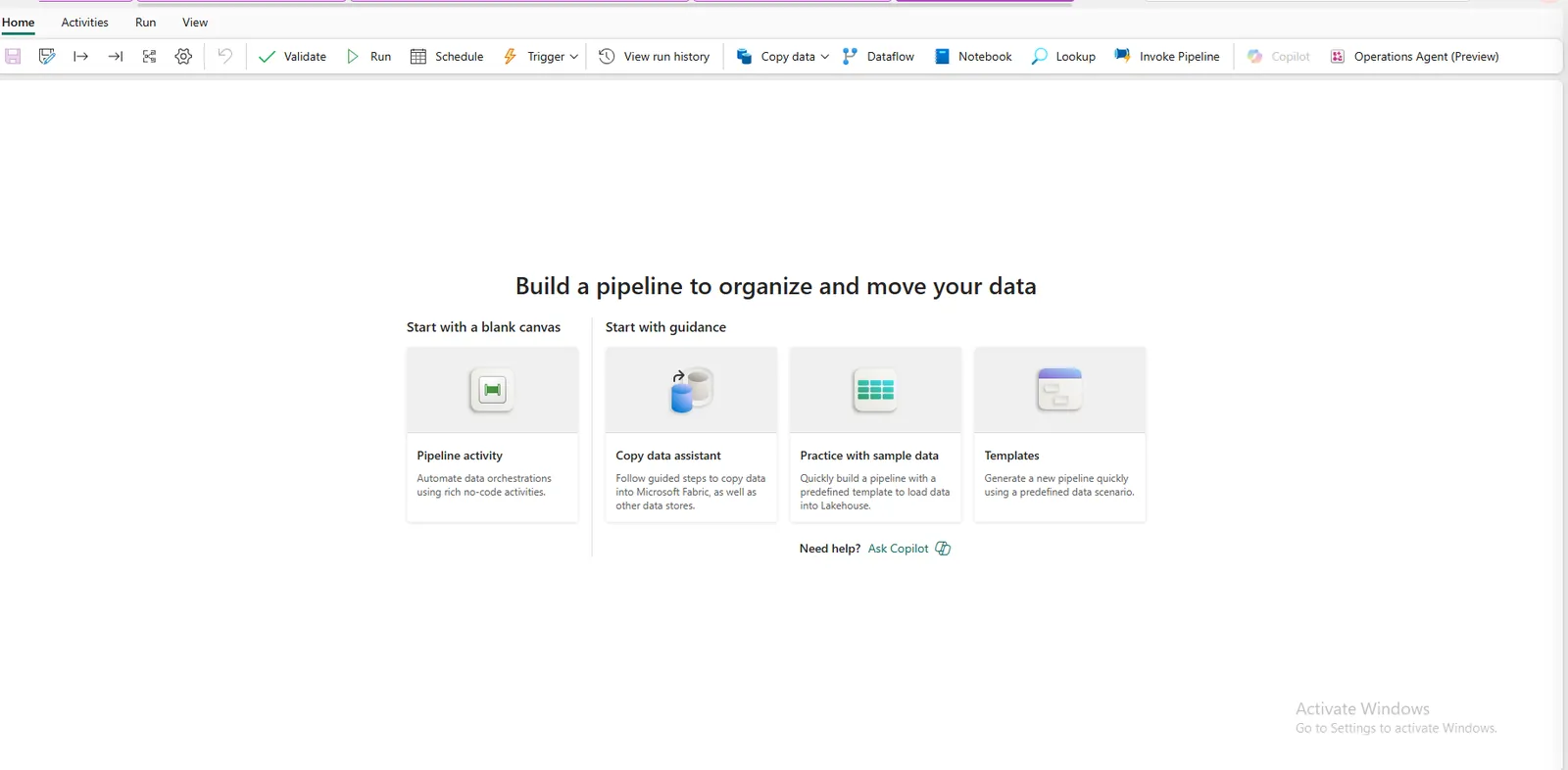
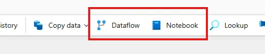
3. In the top ribbon, add the activities:

   • Click Dataflow to add a Dataflow activity.
   • Click Notebook twice to add two Notebook activities.

   

   

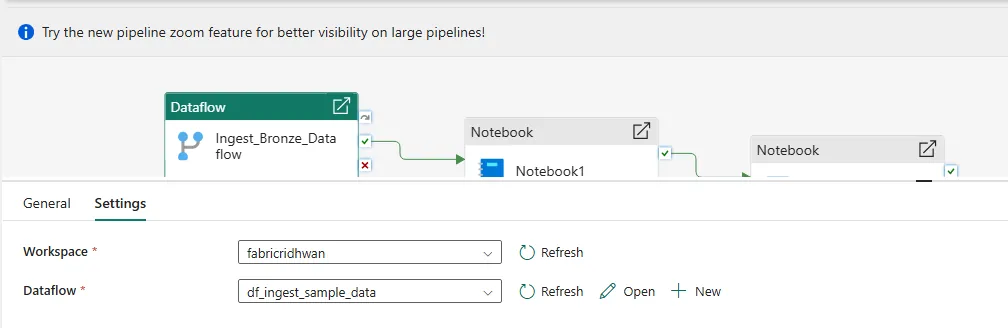
4. Configure Activity 1 (Bronze Ingestion):

   • Name: Ingest_Bronze_Dataflow
   • Settings: Select df_ingest_sample_data

   

5. Configure Activity 2 (Silver Transformation):

   • Name: Transform_Silver_Notebook
   • Settings: Select nb_01_silver_transform
   • Connect: Drag the green checkmark (On Success) from Ingest_Bronze_Dataflow to this activity.

6. Configure Activity 3 (Gold Aggregations):

   • Name: Optimize_Gold_Notebook
   • Settings: Select nb_02_gold_star_schema
   • Connect: Drag the green checkmark (On Success) from Transform_Silver_Notebook to this activity.

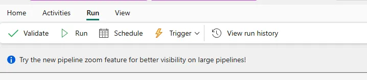
7. Click Validate on the top toolbar to check for errors, then click Run.

   

Troubleshooting Tip: Spark Notebook Concurrency Errors

If your pipeline hangs or fails during notebook execution due to capacity limits on an F2 SKU:

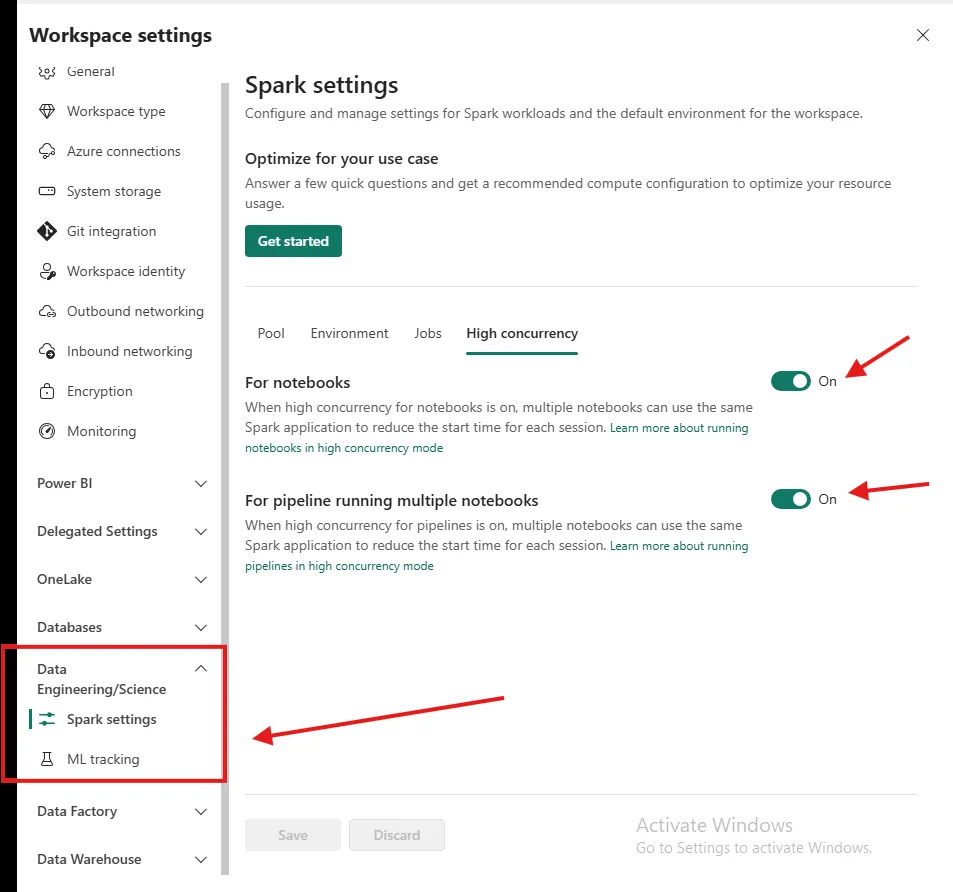
1. Go to Workspace settings → Spark settings.

2. Under High concurrency, enable notebook high concurrency options for pipeline executions. This allows multiple notebook runs to share active Spark sessions without waiting for separate clusters to cold-start.